First Steps in SatMAD: Propagating an Orbit with a TLE

This tutorial illustrates some of the basic functionalities of SatMAD (see the documentation for the latest or more advanced functionalities).

Many of the satellite mission analysis and design problems have four steps:

1. Initialise an orbit

2. Propagate the orbit to generate the trajectory over a duration

3. Do some analysis with this trajectory

4. Plot the results

In this tutorial we will go over these four basic steps to show how SatMAD works.

The first step is to initialise the orbit. For this task we will start with a telecommunications satellite on a geostationary orbit. The up-to-date orbital elements of Turksat-4A can be retrieved from Celestrak website.

from satmad.propagation.tle import TLE

name = "TURKSAT 4A"
line1 = "1 39522U 14007A   20193.17132507  .00000144  00000-0  00000+0 0  9992"
line2 = "2 39522   0.0769 271.0842 0000679 241.5624 240.5627  1.00268861 23480"

tle = TLE.from_tle(line1, line2, name)

print(tle)

TURKSAT 4A
1 39522U 14007A   20193.17132507  .00000144  00000-0  00000+0 0  9992
2 39522   0.0769 271.0842 0000679 241.5624 240.5627  1.00268861 23480

This initialises the orbit from the Two-Line-Element data.

The next step is to propagate the orbit. In this example, we define the propagator sgp4 with an output stepsize of 120 seconds. We then define an interval with a start time and a duration. Finally, we propagate the orbit with gen_trajectory(), taking the inputs of tle (initial orbit) and propagation interval. The output is the trajectory in GCRS coordinate frame.

from satmad.utils.timeinterval import TimeInterval
from satmad.propagation.sgp4_propagator import SGP4Propagator
from astropy import units as u
from astropy.time import Time

# init SGP4
sgp4 = SGP4Propagator(stepsize=120 * u.s)

#  Propagate 3 days into future
interval = TimeInterval(Time("2020-07-11T00:10:00.000", scale="utc"), 3.0 * u.day)
rv_gcrs = sgp4.gen_trajectory(tle, interval)

print(rv_gcrs)

Trajectory from 2020-07-11T00:10:00.000 to 2020-07-14T00:10:00.000 in frame gcrs. (Interpolators initialised: False)

The third step is to do some analysis with this trajectory. In theory, a geostationary orbit is stationary with respect to the rotating Earth. For this simple example, we can check whether this definition holds and how the satellite moves in the Earth-fixed frame.

To this end, we should first convert the internal coordinates data in GCRS to the Earth-fixed (ITRS) coordinates. The next step is to set a reference value and check how much the satellite position deviate in time from this reference position.

Note that the coordinate transformations are handled by Astropy.

# convert GCRS to ITRS
rv_itrs = rv_gcrs.coord_list.transform_to("itrs")

# set reference coordinates and generate position & velocity differences
rv_itrs_ref = rv_itrs[0]

r_diff = (
    rv_itrs.cartesian.without_differentials()
    - rv_itrs_ref.cartesian.without_differentials()
)

v_diff = rv_itrs.velocity - rv_itrs_ref.velocity

# Compute max position and velocity deviation
print(f"Max position deviation: {r_diff.norm().max()}")
print(f"Max velocity deviation: {v_diff.norm().max().to(u.m / u.s)}")

Max position deviation: 81.31617734201691 km
Max velocity deviation: 5.909240646669063 m / s

This shows that the maximum deviation from the reference position was more than 80 km. Similarly, the maximum velocity difference was more than 5 m/s. These are not small differences, and they are actually due to the force model assumptions and orbit maintenance strategy in GEO.

However, we would like to understand these differences a bit more and this necessitates the final step: plotting the results.

from astropy.visualization import time_support
from astropy.visualization import quantity_support
from matplotlib import pyplot as plt

quantity_support()
time_support()

fig1 = plt.figure()
ax1 = fig1.add_subplot(2,1,1)
ax2 = fig1.add_subplot(2,1,2)
plt.suptitle("Departure from Initial Position and Velocity")

fig1.subplots_adjust(hspace=0.5)

ax1.set_ylabel("Pos diff (km)")
ax1.plot(rv_itrs.obstime, r_diff.norm())

ax2.set_ylabel("Vel diff (m/s)")
ax2.plot(rv_itrs.obstime, v_diff.norm().to(u.m / u.s))

plt.show()

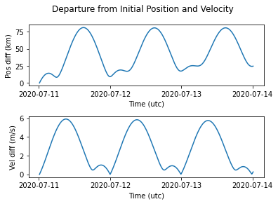
The results show a periodic motion with respect to the initial point, as well as a linear departure.

Perhaps more useful is to see this motion on a latitude-longitude plot, where we can see how geostationary the satellite is. Usually satellite operators define a control box in this coordinate frame and make sure the satellite stays in this box.

from matplotlib.ticker import FormatStrFormatter
from astropy.coordinates import EarthLocation

# Generate lat-lon data
lla = EarthLocation.from_geocentric(
    rv_itrs.cartesian.x, rv_itrs.cartesian.y, rv_itrs.cartesian.z
)

# Show lat-lon plot
fig2, ax = plt.subplots()

ax.grid()
ax.xaxis.set_major_formatter(FormatStrFormatter("% 3.3f"))
ax.yaxis.set_major_formatter(FormatStrFormatter("% 3.3f"))
ax.set_xlabel("Longitude (deg)")
ax.set_ylabel("Latitude (deg)")
ax.plot(lla.lon, lla.lat)
plt.show()

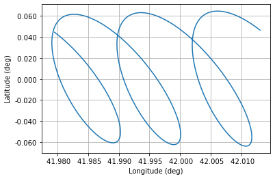
We see further proof that there is a periodic motion as well as a linear drift. Any further analysis is beyond the scope of this simple tutorial.

That said, we have shown the four fundamental steps of approaching a problem with SatMAD: initialisation, propagation, analysis and plotting the results.